Aerodynamic Forces and Simulations

Design for aerodynamics
When most of us hear the term “aerodynamics,” our minds instinctively jump to images of planes soaring in the skies or cars cruising along highways. However, aerodynamics, the science of how air moves around objects, plays a significant role in more everyday objects.

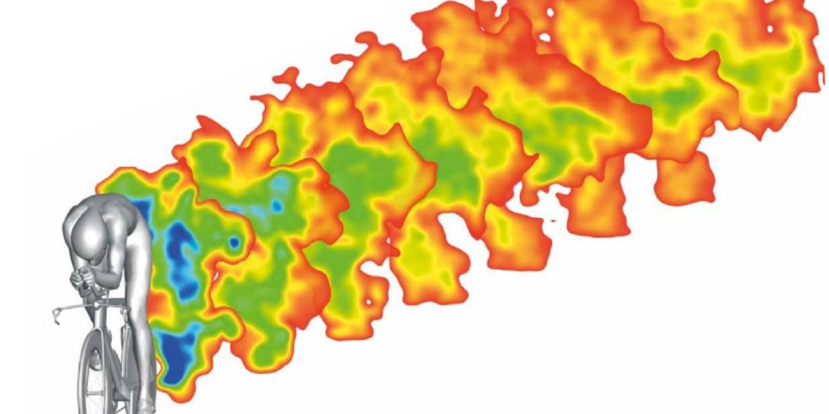
The streamlined designs of racing bikes are more than aesthetics; they are precisely crafted to minimise air resistance. Beyond transportation and sports, the buildings we live and work in are also influenced by aerodynamics. Architects and engineers consider how wind forces might act upon skyscrapers and structures, optimising designs to ensure a favourable wind climate.

Every object interacts with the air in unique ways, experiencing forces that can be advantageous or detrimental. Airplanes offer a clear illustration of the balance involved in aerodynamic design. These aircraft need to generate enough lift (L) in all stages of flight – take-off, cruise and landing. Simultaneously, they aim to reduce drag (D), the opposing force to their forward motion, to ensure fuel efficiency. Finding the perfect balance between these two forces is the challenge. Gliders serve as an exemplary model of optimising this balance. Some modern gliders can fly over 60 kilometres while descending from just 1000-meter of altitude.

Aerodynamic Forces
Intuitively you can imagine that a large truck will experience a bigger resistance in moving through the air than a streamlined, small solar car. How large the difference is can be quantified by calculating the drag around the different shapes. This drag force is defined as follows:

It can be observed from this equation that as an object’s velocity (V) increases, its drag rises exponentially. Hence, as cars or any object speeds up, aerodynamic forces contribute more significantly to total resistance. Consequently, optimising an object’s shape to reduce these forces becomes increasingly important at higher speeds. Reducing drag can be approached in two ways: minimising the frontal area (S) and ensuring smooth airflow around an object, as described by the drag coefficient (Cd).

Lift is calculated in a very similar way:

Where a larger lift force can again be achieved with an increase in velocity (V), area (S) or the lift coefficient (Cl). For instance, the flaps on an airplane, which extend during takeoff or landing, serve to increase the lift coefficient. Likewise, the large rear wing of a Formula 1 race car is designed with a negative lift coefficient, ensuring crucial downforce and grip.

Determining aerodynamic forces
Experimental aerodynamics allows us to measure the forces on a body directly. This can be done by making the air flow around the object, for example in wind tunnels, or by moving the object through the air, with real-world tests. Inside a wind tunnel, a balance captures the forces acting on the object, similar to how a scale measures our weight. In real-world tests with e.g. cars the focus is on energy consumption. For instance, coast-down tests assess how fast a car slows from a set speed; with this data, coupled with information about other forces on the car, aerodynamic forces can be determined.

Historically, these experimental techniques were the norm. But as technology advanced, bringing more computing power and refined numerical methods, simulating air flows around objects has become more common. This evolving domain is known as numerical aerodynamics or computational fluid dynamics (CFD).

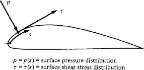
At their core, aerodynamic forces originate from two primary sources: the distribution of pressure and the shear stress over an object’s surface (see image 1 below). The former leads to force acting perpendicular to the surface, reflecting how the air exerts pressure on the object. The latter, the shear stress, operates tangentially, resulting from friction between the air and the object. A smooth surface like glass will have less friction than a rough surface like sandpaper.

To numerically compute the aerodynamic forces, these distributions must be integrated across the object’s surface. This involves dividing the surface into small areas and then summing the contributions of pressure and shear stress. All the components in the horizontal direction add up to the drag force, the components in the vertical direction contribute to the lift force.

The determination of the forces in this way is only possible when the pressure and shear stress distributions are known over the surface of an object. How this is achieved with CFD is described in the next section.

The basics of CFD
Fundamental equations
At the basis of CFD lie fundamental principles that are always valid also outside the field of aerodynamics. These principles are:
– Conservation of mass; mass cannot be created nor destroyed
– Conservation of momentum, derived from Newton’s second law: Force = mass x acceleration
– Conservation of energy; energy cannot be created nor destroyed, it can only change from one form to another

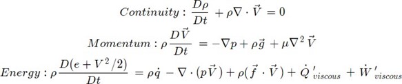
These fundamental principles can be used to derive the governing flow equations for continuity, momentum and energy as shown below, also known as the Navier Stokes Equations. They are merely shown as illustration as the detailed explanation goes beyond the scope of this essay.

Discretization of the problem
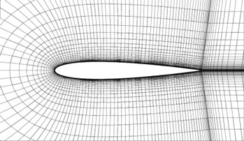
Real-world fluid problems are continuous. However, computers can only work with discrete data. Therefore, the continuous flow field around an object needs to be broken down or “discretized” into smaller solvable parts. The distribution of the flow field into smaller pieces, also called cells, yields a mesh. A 2D mesh around a wing profile is shown in the image 2 below. The cells close to the surface of the wing are smaller, since the largest changes in flow are expected there and therefore more cells are needed to capture the details.

To be able to solve the Navier Stokes equations in these cells, they must be converted into an algebraic form. This discretization can be achieved with different methods where the solution in a cell is dependent on the variables of the neighbouring cells. Discretizing inevitably approximates the equations, introducing slight errors. The accuracy of these discretization techniques varies, with more accurate methods typically demanding more time for computation.

Modelling turbulence
You could imagine that solving smooth and orderly airflow will be easier than random and chaotic flow. However, the latter, called turbulent flow, is quite common: around car wheels, behind windmills or surrounding buildings. The Navier-Stokes equations inherently account for turbulence. However, directly resolving all the scales of turbulence, from the largest energy-containing eddies down to the smallest dissipative scales, requires a lot of computational resources. Instead, various models have been developed to approximate the effects of turbulence. This approach allows for the simulation of turbulent flows without directly resolving every detail, making it possible to study complex turbulent flows with available computational resources.

Again, the approaches differ in e.g. accuracy, applicability and time to solve. A widely used approach is the Reynolds-Averaged Navier-Stokes (RANS) method, where the turbulence is modelled with a mean and a fluctuating term. With this method a time-averaged solution is achieved without detailing time-dependent flow behaviours. The RANS simulation can be solved relatively fast and the accuracy is sufficient for most applications. When flows become very chaotic or complex, this method is not the preferred choice. Other, more accurate and computational heavier methods should be used.

Solving the equations
The solving part in CFD starts with an initial guess of the flow variables and the solution is improved iteratively. Every iteration the solution of the previous iteration is used to calculate the new flow properties. Whether the simulation has converged to a solution is typically checked by monitoring residuals, which are a measure of the imbalance in the solved equations. Once residuals drop below a set threshold, the solution is converged to the final solution.

Results
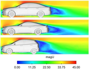
With the resulting pressure and shear stress distributions, the aerodynamic forces can be calculated. Next to these forces, the results of a CFD simulation can be represented by images of the flow field around an object. For example, the pressure field over a wing profile or the velocity field around a car (see image 3 below). The red area over the roof of the cars shows an increase in velocity, while behind the car the velocity is low in the blue area. This low velocity region behind the car is called the wake and gives an indication of the drag force on the car. Usually the smaller this blue region, the lower the drag. These visual results can offer a deeper understanding about the aerodynamic efficiency of a design, a perspective that is more challenging to achieve in wind tunnel experiments.

Final remarks
Navigating the world of CFD isn’t as straightforward as plugging in values and waiting for results. Given the countless options of methods, models, and the requirements for a robust computational mesh, users must have a good understanding of the applicable assumptions to ensure meaningful results. CFD is therefore not the solution to all aerodynamic problems, but rather a part of the toolbox next to analytical methods and wind tunnel experiments. The application of all these tools allows us to design objects for optimal aerodynamics.

References:
Throughout the essay reference [1] was consulted.
[1] Anderson, John D., Jr.: Fundamentals of Aerodynamics (4th Edition), McGraw-Hill, New York, 2007.
[2] Rahman, Md & Agarwal, Ramesh & Lampinen, Markku & Siikonen, Timo. An Improved Version of One-Equation RAS Turbulence Model. 45th AIAA Fluid Dynamics Conference, 2015.
[3] Lietz, Robert & Larson, Levon & Bachant, Pete & Goldstein, John & Silveira, Rafael & Shademan, Mehrdad & Ireland, Pete & Mooney, Kyle. An Extensive Validation of an Open Source Based Solution for Automobile External Aerodynamics, WCX™ 17: SAE World Congress Experience, 2017.